import geopandas as gpd
from pathlib import Path3 Introduction to vector data
Now we’ll look at the second main type of data - vector data. You will be able to:
- Describe the strengths and weaknesses of storing data in vector format.
- Describe the different types of vectors and identify types of data that would be stored in each.
- Use GeoPandas to read and work with a vector data file in Shapefile format.
3.1 Readings and resources
3.2 About vector data
Vector data structures represent specific features on the Earth’s surface, and assign attributes to those features. Vectors are composed of discrete geometric locations (x, y values) known as vertices that define the shape of the spatial object. The organization of the vertices determines the type of vector that we are working with: point, line or polygon.
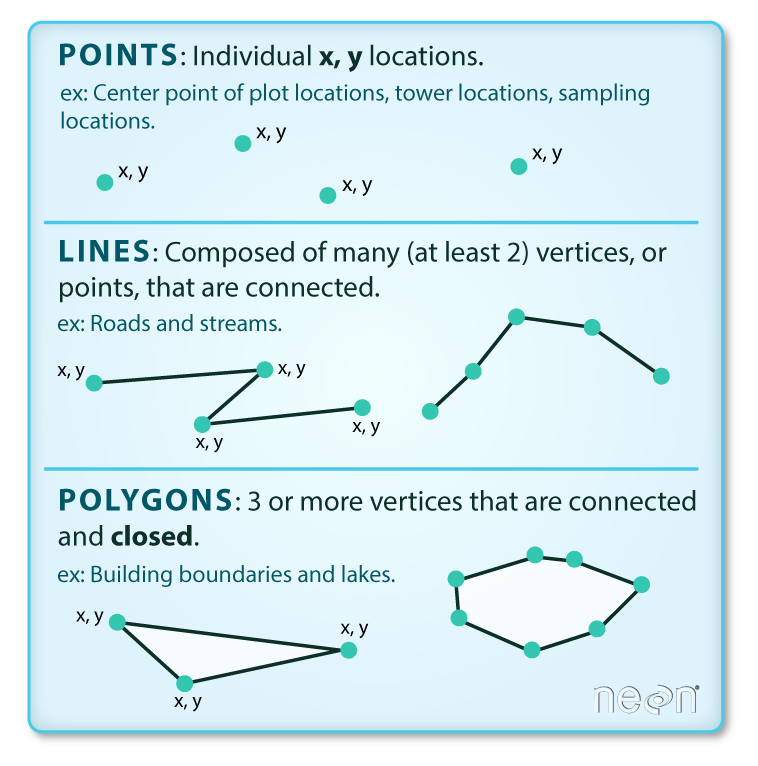
Points: Each point is defined by a single x, y coordinate. There can be many points in a vector point file. Examples of point data include: sampling locations, the location of individual buildings, or the location of bathrooms.
Lines: Lines are composed of many (at least 2) points that are connected. For instance, a road or a stream may be represented by a line. This line is composed of a series of segments, each “bend” in the road or stream represents a vertex that has a defined x, y location.
Polygons: A polygon consists of 3 or more vertices that are connected and closed. The outlines of survey plot boundaries, lakes, oceans, and states or countries are often represented by polygons.
Data Tip
Sometimes, boundary layers such as states and countries, are stored as lines rather than polygons. However, these boundaries, when represented as a line, will not create a closed object with a defined area that can be filled.
Challenge - Identify Vector Types
The plot below includes examples of two of the three types of vector objects. Use the definitions above to identify which features are represented by which vector type.
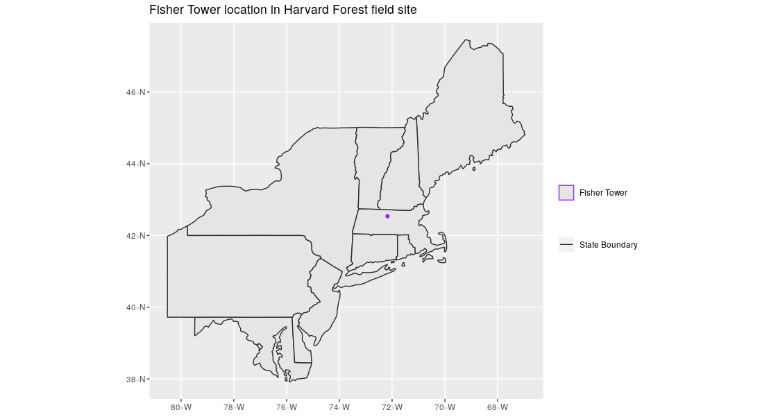
Solution
State boundaries are polygons. The Fisher Tower location is a point. There are no line features shown.
Vector data has some important advantages:
- The geometry itself contains information about what the dataset creator thought was important.
- The geometry structures hold information in themselves - why choose point over polygon, for instance?
- Each geometry feature can carry multiple attributes instead of just one, e.g. a database of cities can have attributes for name, country, population, etc.
- Data storage can be very efficient compared to rasters. For example, a polygon of a large area can be represented with a small number of vertices as compared to all the raster grid elements making up the polygon.
The downsides of vector data include:
- Potential loss of detail compared to raster.
- Potential bias in datasets - what didn’t get recorded?
- Calculations involving multiple vector layers need to do math on the geometry as well as the attributes, so can be slow compared to raster math.
Vector datasets are in use in many industries besides geospatial fields. For instance, computer graphics are largely vector-based, although the data structures in use tend to join points using arcs and complex curves rather than straight lines. Computer-aided design (CAD) is also vector-based. The difference is that geospatial datasets are accompanied by information tying their features to real-world locations.
3.3 Important attributes of vector data
3.3.1 Extent
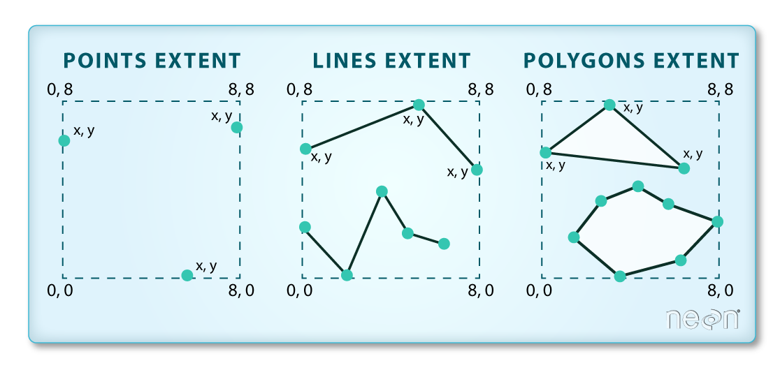
The spatial extent is the geographic area that the geographic data covers. The spatial extent of an object represents the geographic edge or location that is the furthest north, south, east and west. In other words, extent represents the overall geographic coverage of the spatial object.
Challenge - Extent
In the image above, the dashed boxes around each set of objects seems to imply that the three objects have the same extent. Is this accurate? If not, which object(s) have a different extent?
Solution
The lines and polygon objects have the same extent. The extent for the points object is smaller in the vertical direction than the other two because there are no points on the line at y = 8.
3.4 Vector data format for this module
Like raster data, vector data can also come in many different formats. For this module, we will start with the Shapefile format. This is an extremely common (and old) format developed by ESRI the company behind the most popular commercial GIS package, ArcGIS.
A Shapefile format consists of multiple files in the same directory, of which .shp, .shx, and .dbf files are mandatory. Other non-mandatory but very important files are .prj and shp.xml files.
- The
.shpfile stores the feature geometry itself .shxis a positional index of the feature geometry to allow quickly searching forwards and backwards through the geographic coordinates of each vertex in the vector.dbfcontains the tabular attributes for each shape. Based on the really old (1983, pre-Windows), dBASE, file format..prjfile indicates the coordinate reference system (CRS).shp.xmlcontains the Shapefile metadata.
Together, the Shapefile includes the following information:
- Extent - the spatial extent of the shapefile (i.e. geographic area that the shapefile covers). The spatial extent for a shapefile represents the combined extent for all spatial objects in the shapefile.
- Object type - whether the shapefile includes points, lines, or polygons.
- Coordinate reference system (CRS) - more on this later.
- Other attributes - for example, a line shapefile that contains the locations of streams, might contain the name of each stream.
Because the structure of points, lines, and polygons are different, each individual shapefile can only contain one vector type (all points, all lines or all polygons). You will not find a mixture of point, line and polygon objects in a single shapefile.
Later in this module we’ll look at GeoJSON files, another format for storing vector data.
3.5 Integrated raster and vector data formats
Very few formats can contain both raster and vector data - in fact, most are even more restrictive than that. Vector datasets are usually locked to one geometry type, e.g. points only. Raster datasets can usually only encode one data type, for example you can’t have a multiband GeoTIFF where one layer is integer data and another is floating-point. There are sound reasons for this - format standards are easier to define and maintain, and so is metadata. The effects of particular data manipulations are more predictable if you are confident that all of your input data has the same characteristics.
There are integrated file formats that do allow you to mix separate vector and raster files within the same container file. These include GeoPackage (which is a SQLite database) and Geodatabase formats.
How might we store and use vector data in Python?
3.6 Add geospatial functionality to pandas
The basic idea behind GeoPandas is to combine the capabilities of pandas with the shapely library to allow you to work with geospatial data in a pandas-like way.
GeoPandas is an open source project to make working with geospatial data in python easier. GeoPandas extends the datatypes used by pandas to allow spatial operations on geometric types. Geometric operations are performed by shapely. GeoPandas further depends on fiona for file access and matplotlib for plotting.
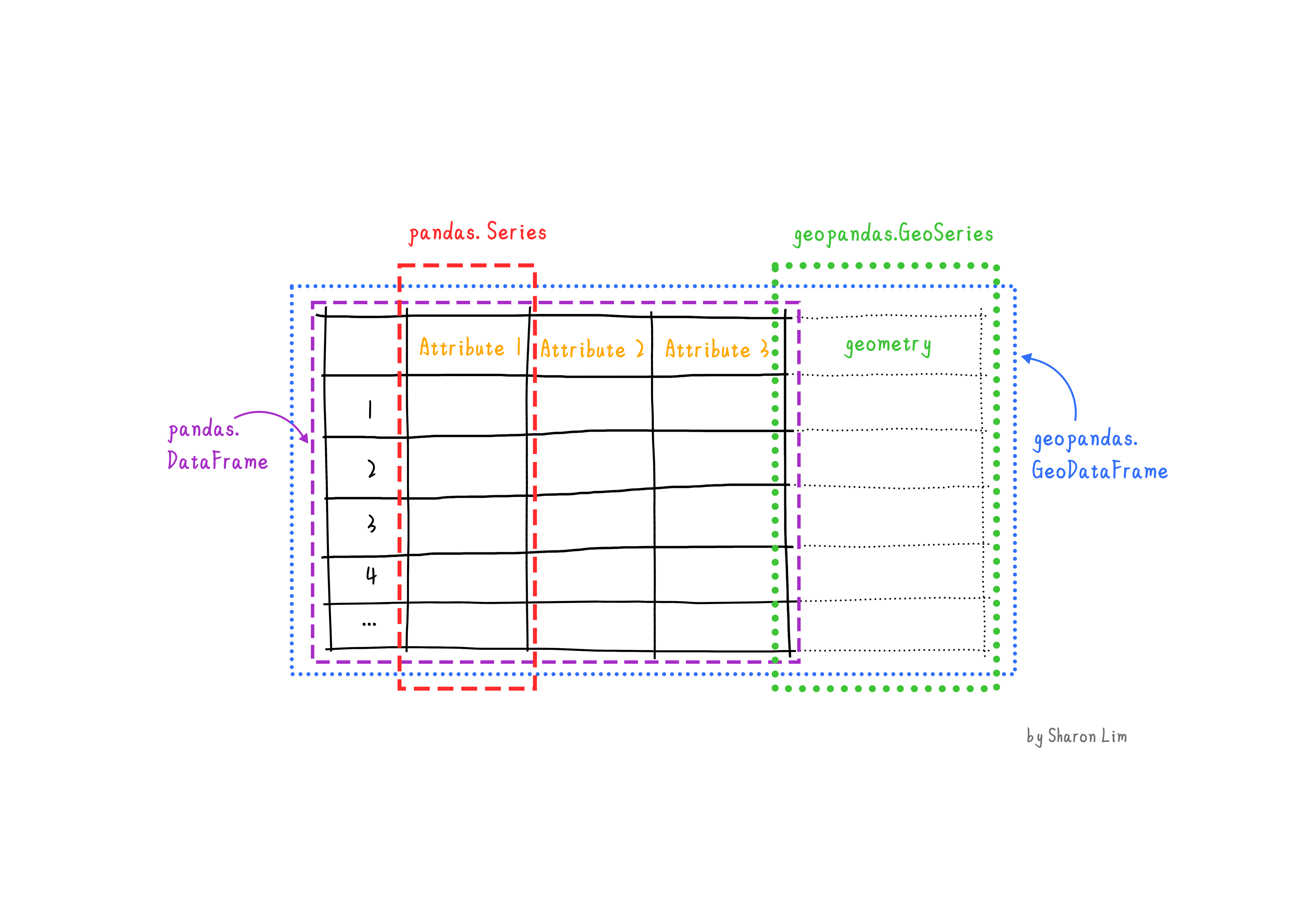
GeoPandas extends the popular pandas library for data analysis to geospatial applications. The main pandas objects (the Series and the DataFrame) are expanded to geopandas objects (GeoSeries and GeoDataFrame). This extension is implemented by including geometric types, represented in Python using the shapely library, and by providing dedicated methods for spatial operations (union, intersection, etc.). The relationship between Series, DataFrame, GeoSeries and GeoDataFrame can be briefly explained as follow:
- A
Seriesis a one-dimensional array with axis, holding any data type (integers, strings, floating-point numbers, Python objects, etc.) - A
DataFrameis a two-dimensional labeled data structure with columns of potentially different types1. - A
GeoSeriesis aSeriesobject designed to store shapely geometry objects. - A
GeoDataFrameis an extendedpandas.DataFrame, which has a column with geometry objects, and this column is aGeoSeries.
Let’s use geopandas to read a shapefile. The US government provides Cartographic Boundary Files in both geodatabase and shapefile formats. They are available at different levels of resolution and also by geographic region.
The cartographic boundary files are simplified representations of selected geographic areas from the Census Bureau’s Master Address File/Topologically Integrated Geographic Encoding and Referencing (MAF/TIGER) System. These boundary files are specifically designed for small scale thematic mapping. As of 2019, cartographic boundary files are available in shapefile, geodatabase, and Keyhole Markup Language (KML) format. For more details about these files, including their appropriate usage, please see our Cartographic Boundary File Description page.
From this link, I downloaded a zipped shapefile (cb_2022_26_place_500k.zip) for the Places in the state of Michigan. As we’ll see, these are things like city and township boundaries. After uncompressing it, the resulting folder looks like this:
├── cb_2022_26_place_500k
│   ├── cb_2022_26_place_500k.cpg
│   ├── cb_2022_26_place_500k.dbf
│   ├── cb_2022_26_place_500k.prj
│   ├── cb_2022_26_place_500k.shp
│   ├── cb_2022_26_place_500k.shp.ea.iso.xml
│   ├── cb_2022_26_place_500k.shp.iso.xml
│   └── cb_2022_26_place_500k.shx
└── cb_2022_26_place_500k.zip

1 directory, 8 files
Now let’s open the shapefile with geopandas.
To read a shapefile, we can use the read_file() function and pass in the name of the file with the .shp extension.
mi_places_file = Path('data', 'cb_2022_26_place_500k', 'cb_2022_26_place_500k.shp')
mi_places_gdf = gpd.read_file(mi_places_file)

mi_places_gdf.info()
<class 'geopandas.geodataframe.GeoDataFrame'>
RangeIndex: 745 entries, 0 to 744
Data columns (total 13 columns):
# Column Non-Null Count Dtype
--- ------ -------------- -----
0 STATEFP 745 non-null object
1 PLACEFP 745 non-null object
2 PLACENS 745 non-null object
3 AFFGEOID 745 non-null object
4 GEOID 745 non-null object
5 NAME 745 non-null object
6 NAMELSAD 745 non-null object
7 STUSPS 745 non-null object
8 STATE_NAME 745 non-null object
9 LSAD 745 non-null object
10 ALAND 745 non-null int64
11 AWATER 745 non-null int64
12 geometry 745 non-null geometry
dtypes: geometry(1), int64(2), object(10)
memory usage: 75.8+ KBThe resulting data structure is called a GeoDataFrame. In addition to standard DataFrame fields, a GeoDataFrame has one or more geometry fields. Only one geometry field is considered active at any one time. As you might guess, this field will allow us to do spatial queries with pandas-like commands as well as plot the data.
Let’s see what’s in the geometry field.
mi_places_gdf[['NAME', 'geometry']].head(15)| NAME | geometry | |
|---|---|---|
| 0 | Wakefield | POLYGON ((-89.98990 46.47580, -89.98972 46.477... |
| 1 | Hesperia | POLYGON ((-86.04946 43.57584, -86.03964 43.575... |
| 2 | Britton | POLYGON ((-83.84044 41.98837, -83.83784 41.987... |
| 3 | Zilwaukee | POLYGON ((-83.93590 43.47955, -83.93557 43.494... |
| 4 | Zeeland | POLYGON ((-86.03850 42.80958, -86.03564 42.812... |
| 5 | Sunfield | POLYGON ((-85.00503 42.76676, -84.98533 42.766... |
| 6 | Suttons Bay | POLYGON ((-85.65931 44.98558, -85.65684 44.985... |
| 7 | Big Rapids | POLYGON ((-85.50392 43.68804, -85.50381 43.695... |
| 8 | Fife Lake | POLYGON ((-85.36328 44.57706, -85.36324 44.580... |
| 9 | Bloomfield Hills | POLYGON ((-83.26587 42.59630, -83.25753 42.596... |
| 10 | Tustin | POLYGON ((-85.46393 44.10665, -85.45380 44.106... |
| 11 | Melvin | POLYGON ((-82.87187 43.19339, -82.85227 43.193... |
| 12 | Roosevelt Park | POLYGON ((-86.28329 43.20215, -86.28320 43.205... |
| 13 | Hudson | POLYGON ((-84.36191 41.86440, -84.36097 41.863... |
| 14 | North Branch | POLYGON ((-83.21524 43.22503, -83.20216 43.225... |
As each row is a “place” in Michigan, it’s not surprising to find POLYGON objects in the geometry field. You’ll explore this GeoDataFrame further in the land use analysis notebook below.
3.7 Case Study: Land use analysis on the OU campus
For this this module, you’ll be working through a Jupyter notebook that introduces the very basics of working with vector data in shapefile format.
3.7.1 Activities
Launch Jupyter lab and open the ou_land_use_02_vectorintro.ipynb file. Work your way through it.