2 Introduction to raster data
There are two primary data types that we will learn about for storing geospatial data - raster and vector data. We will start out learning about raster data. You will be able to:
- Describe the difference between raster and vector data.
- Describe the strengths and weaknesses of storing data in raster format.
- Distinguish between continuous and categorical raster data and identify types of datasets that would be stored in each format.
2.1 Readings and resources
- GCwP - Ch 1: Geographic Data in Python - Section 1.3
- GCwR - Ch 2: Geographic Data in R - Section 2.3
- GIS Stack Exchange is like StackOverflow for geospatial questions. Very helpful.
Yes, I know this class is Python based, but I’m including the second reference for a few reasons. First of all, it has outstanding, well written, content. Secondly, R has many strengths for geospatial analysis and mapping and most of you have already learned both R and Python basics in my previous course. It’s good to be aware of the R ecosystem for geocomputation as then you can pick and choose your tools as you see fit. R and Python are becoming more interoperable as time goes on and mixing the two is becoming quite common.
2.2 Data structures: raster and vector
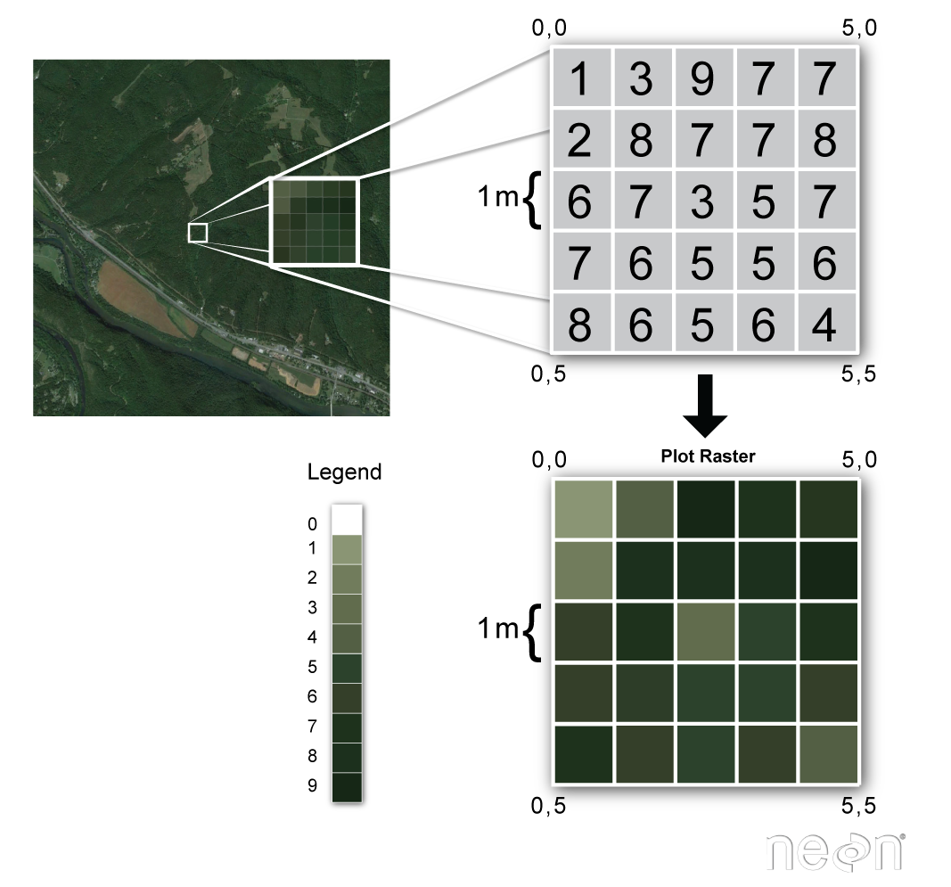
The two primary types of geospatial data are raster and vector data. Raster data is stored as a grid of values which are rendered on a map as pixels. Each pixel value represents an area on the Earth’s surface. Vector data structures represent specific features on the Earth’s surface (e.g. boundaries, bodies of water, roads, buildings, dams, parks, …), and assign attributes to those features. Vector data structures will be discussed in more detail in Chapter 3.
This module will focus on how to work with both raster and vector data sets, therefore it is essential that we understand the basic structures of these types of data and the types of data that they can be used to represent. Many maps have a combination of vector and raster data. For example, when you use satellite view in Google Maps, you are seeing vector data such as roads and places layered on top of aerial imagery which is raster data.
2.3 About raster data
Raster data is any pixelated (or gridded) data where each pixel is associated with a specific geographic location. The value of a pixel can be continuous (e.g. elevation) or categorical (e.g. land use). If this sounds familiar, it is because this data structure is very common: it’s how we represent any digital image. A geospatial raster is only different from a digital photo in that it is accompanied by spatial information that connects the data to a particular location. This includes the raster’s extent (the area represented by the raster), cell size, the number of rows and columns, and its coordinate reference system (or CRS).
Some examples of continuous rasters include:
- Precipitation maps,
- Maps of tree height derived from lidar data,
- Elevation values for a region.
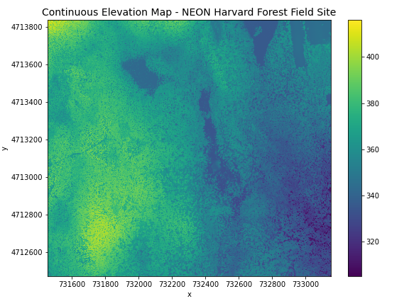
A map of elevation for Harvard Forest derived from the NEON AOP LiDAR sensor is below. Elevation is represented as a continuous numeric variable in this map. The legend shows the continuous range of values in the data from around 300 to 420 meters.
Some rasters contain categorical data where each pixel represents a discrete class such as a landcover type (e.g., “forest” or “grassland”) rather than a continuous value such as elevation or temperature. Some examples of classified maps include:
- Landcover / land-use maps,
- Tree height maps classified as short, medium, and tall trees.
- Elevation maps classified as low, medium, and high elevation.
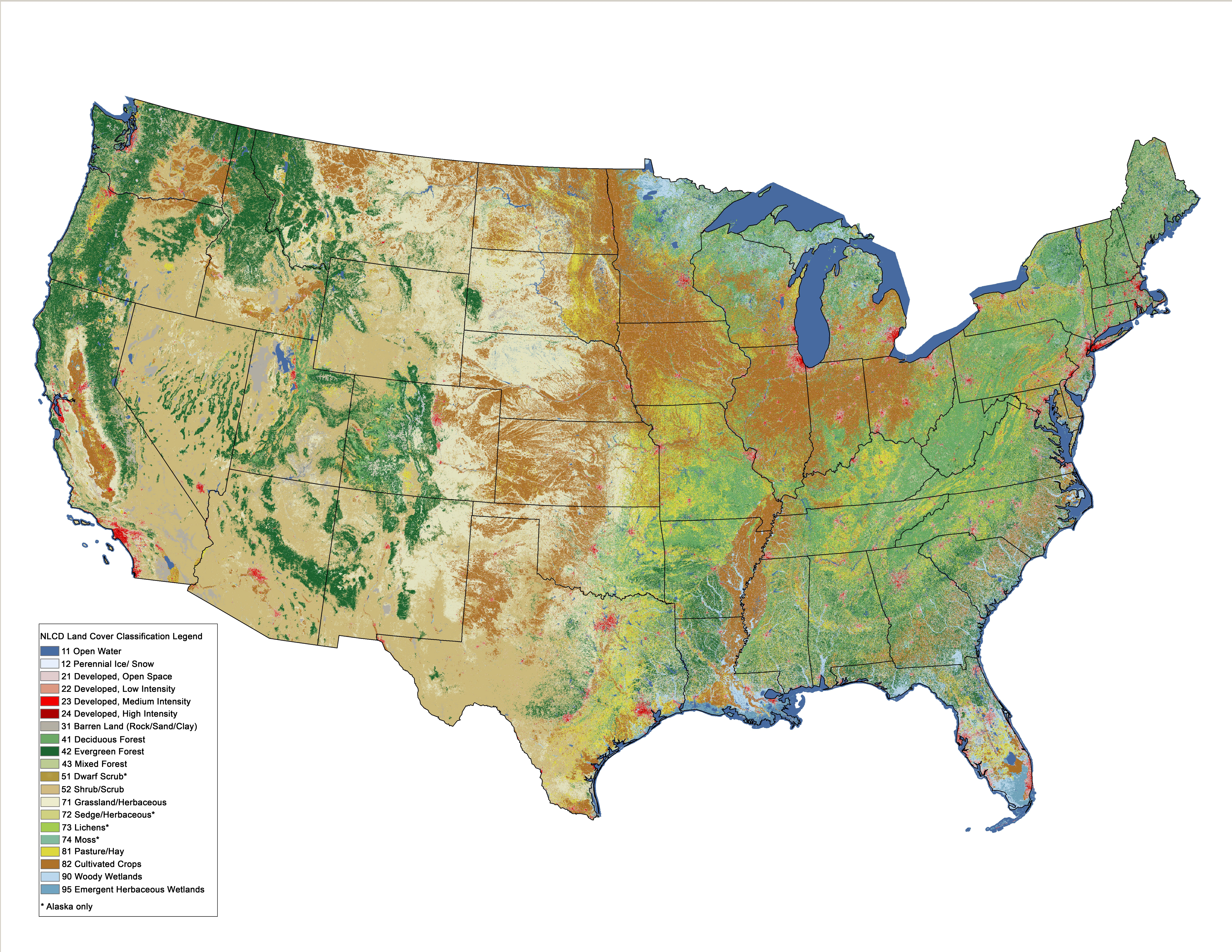
The map above shows the contiguous United States with landcover as categorical data. Each color is a different landcover category. (Source: Homer, C.G., et al., 2015, Completion of the 2011 National Land Cover Database for the conterminous United States-Representing a decade of land cover change information. Photogrammetric Engineering and Remote Sensing, v. 81, no. 5, p. 345-354)
Think about potential advantages and disadvantages of storing data in raster format and list them.
Raster data has some important advantages:
- representation of continuous surfaces
- potentially very high levels of detail
- data is ‘unweighted’ across its extent - the geometry doesn’t implicitly highlight features
- cell-by-cell calculations can be very fast and efficient
The downsides of raster data are:
- very large file sizes as cell size gets smaller
- currently popular formats don’t embed metadata well (more on this later!)
- can be difficult to represent complex information
2.4 Important attributes of raster data
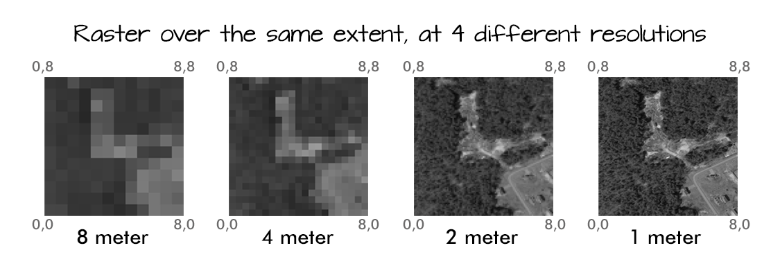
2.4.1 Resolution
A resolution of a raster represents the area on the ground that each pixel of the raster covers. The image below illustrates the effect of changes in resolution.
2.5 Raster data format for this module
Raster data can come in many different formats. We will use the GeoTIFF format which has the extension .tif. A .tif file stores metadata or attributes about the file as embedded tif tags along with the actual raster data. For instance, your camera might store a tag that describes the make and model of the camera or the date the photo was taken when it saves a .tif. A GeoTIFF is a standard .tif image format with additional spatial (georeferencing) information embedded in the file as tags. These tags should include the following raster metadata:
- Extent
- Resolution
- Coordinate Reference System (CRS) - we will introduce this concept in Chapter 4.
- Values that represent missing data (
NoDataValue)
We will discuss these attributes in more detail in later sections.
2.6 Multi-band raster data
A raster can contain one or more bands. One type of multi-band raster dataset that is familiar to many of us is a color image. A basic color image consists of three bands: red, green, and blue. Each band represents light reflected from the red, green or blue portions of the electromagnetic spectrum. The pixel brightness for each band, when composited creates the colors that we see in an image.
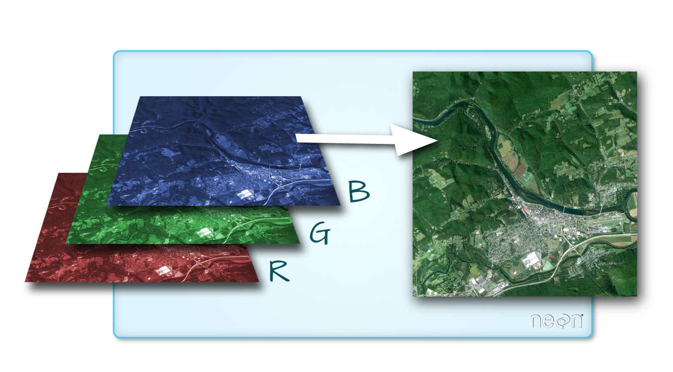
We can plot each band of a multi-band image individually. Or, we can composite all three bands together to make a color image. In a multi-band dataset, the individual band rasters will always have the same extent, resolution, and CRS.
Multi-band raster data might also contain:
- Time series: the same variable, over the same area, over time.
- Multi or hyperspectral imagery: image rasters that have 4 or more (multi-spectral) or more than 10-15 (hyperspectral) bands. We won’t be working with this type of data in this module, but you can check out the NEON Data Skills Imaging Spectroscopy HDF5 in R tutorial if you’re interested in working with hyperspectral data cubes.
- Raster data is pixelated data where each pixel is associated with a specific location.
- Raster data always has an extent and a resolution.
- The extent is the geographical area covered by a raster.
- The resolution is the area covered by each pixel of a raster.
2.7 Case Study: Land use analysis on the OU campus
Throughout this module, we will use this case study to allow you to get some hands on practice with the topics covered. For this first module, you’ll be working through a Jupyter notebook that introduces the overall case study and gives you an introduction to working with relevant raster data representing land use on the OU campus. You’ll get your first look at two import Python packages for working with raster data - xarray and rioxarray.
2.7.1 xarray - labelled multidimension arrays
Xarray builds on top of NumPy N-d arrays and adds the ability to create and work with labels for the dimensions.
Xarray makes working with labelled multi-dimensional arrays in Python simple, efficient, and fun!
The two main data structures are DataArray (a N-d generalization of a pandas.Series) and DataSet (an N-d generalization of a pandas.DataFrame). The Overview: Why xarray? page has a nice level of detail on the case for xarray and its link to geospatial analysis.
2.7.2 rioxarray - read raster data into xarray objects
The rioxarray package extends the xarray package to facilitate reading raster data into xarray objects. The actual reading of the raster file is done using another Python package known as rasterio. Once you load rioxarray, your can use the rio accessor with xarray objects to access rioxarray methods for working with raster data. From the rasterio docs:
Geographic information systems use GeoTIFF and other formats to organize and store gridded raster datasets such as satellite imagery and terrain models. Rasterio reads and writes these formats and provides a Python API based on Numpy N-dimensional arrays and GeoJSON.
2.7.3 Activities
I have created one compressed archive which contains the Jupyter notebook(s) as well as any data (or other) files needed.
Start by downloading the following file and extract it in a location of your choice.
Launch Jupyter lab and open the ou_land_use_01_rasterintro.ipynb file. Work your way through it.
- Download: ou_land_use_analysis.zip